Robust Chessboard Recognition Part 4: A Solution

In the Part 1 of this series, I showed how to turn chessboard recognition into an optimization problem. In Part 2, I discussed different ways of solving this optimization problem, deciding on a custom evolutionary algorithm with tailored mutation operators described in Part 3.   In this post, I discuss my solution. A video of the final solution is shown to the right.

Basic Solution

The last three posts developed the chessboard recognition problem as an optimization problem to be solved by an evolutionary algorithm using specialized mutation operators. So given the score function that assigns a score to possible quadrilaterals as chessboard boundaries, this simple algorithm works as follows. First, a population of 100 quadrilaterals is generated by placing a virtual camera at a random positions around an imaginary chessboard and projecting the chessboard into the camera's frustrum. Then the following steps are repeated one hundred times:

1. Each quadrilateral in the population is scored.
2. The quadrilateral with the highest score is chosen; for this purpose the best quadrilateral from the last population is included, so that selection is elitist.
3. The best quadrilateral is mutated using the tailored mutation operations to generate a new population of 10 quadrilaterals.

After one hundred repetitions (generations) of this form, the best quadrilateral is returned as the algorithms' best guess of at the chessboard location. This quadrilateral is the best out of 1,090 possible quadrilaterals searched. This basic algorithm runs in less than 10 seconds on an Intel i7 processor with support from an nVidia 780ti GPU.

An Elitist Island Model

Although the basic solution works well, it sometimes gets stuck. This problem can be alleviated by running the basic algorithm several times in a distributed fashion. So when the chessboard detection system first starts, it runs the basic algorithm eight times in eight separate processes. Then each one of the eight instance of the algorithm returns a proposed solution. These eight solutions are compared using the score function, but with the addition of a score component that checks the color of the different board positions, which is too expensive to check for all 8,000 possible solutions. The best out of these eight solutions is chosen as the current best guess at the chessboard location for one time step. It takes 10-20 seconds to compute this guess.

Then, for subsequent time steps, four smaller evolutionary algorithms are run. Rather than generating new chessboards from random camera positions, each algorithm is seeded with the initial guess, and generates a new population of ten quadrilaterals just as in Step 3 above. The algorithm is run for just ten more generations, and then the four best quadrilaterals for each evolutionary algorithm are compared again. Once again, the color information is also checked, and the best quadrilateral is published as the current chessboard guess. These smaller evolutionary runs are run in parallel and complete within 250 milliseconds. So after initialization, the entire model runs at 4 Hz, publishing four successive guesses at the chessboard per second.  

An algorithm of this form is called an island model. Each distributed evolutionary algorithm is called an island, and when information travels between islands it is called migration. Island models can be very effective because they maintain some diversity across all islands while allowing a focused search on each island. In this case, our island model is elitist, because when the islands exchange information, it wipes out the past entirely.

Adapting to Change

One of the nice things about an evolutionary algorithm is that it adapts easily to change. If the board is moved while the board detector is running, it only takes a few cycles (5-10 seconds) for the best chessboard guess to adapt to the new reality. While this latency is not fast enough to allow the robot to move its eyes while tracking the board, it is good enough to adjust reasonably if someone accidentally (or intentionally) bumps into the board.

Also, in order to promote stability when the board does not change, it makes sense to keep old detected intersection points, since the lines and intersections detected at each frame may vary. In my approach, old intersection points are rolled off every 5 frames. This is enough to make the board detection robust, for example when an hand is placed between the camera and the board. You can see an example of this in the video above.

Overall Results

The overall solution is very robust and relatively fast. The image to the right shows what a converged example looks like, and the video above shows how the detection adjusts when the board is obscured or moved.

Robust Chessboard Recognition, Part 3: Tailored Mutation Operators

A correctly detected chessboard

In the last two posts, I discussed the chessboard recognition problem and the types of algorithms we could use to solve it. In this post I will describe the solution I developed. As described in the first post, I use an image of the chessboard taken from the iCub's eye, extract lines and intersections, and create a chessboard scoring function that takes a proposed quadrilateral, warps the image to undo the perspective, and then checks to see how many lines and intersections match what is expected from a chessboard. An example of a good quadrilateral is shown to the right.

In the second post, I argued the case for using a simple evolutionary algorithm with custom mutation operators tailored to look for chessboards. In this post, I will describe the mutation operators. In the next post, I'll describe an elitist distributed island model used to select the best chessboard candidates.

Rectangle Mutation

A randomly generated quadrilateral

The general idea is that we start with a quadrilateral with a decent score, and we want to change in a way that might make it better. At the very beginning, the quadrilaterals are chosen by using a projective model from a camera whose position and orientation are somewhat random above and around the chessboard. This projection generates some random convex quadrilaterals. An example is shown to the left. So let's think about what could be wrong with our quadrilateral, and how we could adjust to quadrilateral to fix it.

Snapping Corners to Points

Leftmost corner snapped to point

Looking at the chessboard in the real image above, we notice that the generated quadrilateral has no relationship the to the lines (in red) and intersections (white circles) that we computed for the scoring function. Ideally, the right quadrilateral should have corners that are near intersections on the chessboard. So one of the first mutations we might consider is to snap a corner of the quadrilateral to some intersection that we detected. An example of what happens after this is done is shown to the right. It looks like we have now have nearly matched near the upper left corner of the real chessboard. The image on the right was generated by just ten trial points. 

Top right snapped to point

This snapping operation works because there is a concentration of intersection points inside or near the chessboard, so with high probability we'll pick a point right around the chessboard, and there is a decent probability that we will get a snap point closer to one of the corners. If we do it again, the we might get a second corner a bit closer. This is shown to the right. The snap point actually came from the keyboard. But it doesn't matter, since it got us closer to the right answer.  Again, I only had to sample 10 snap points to get the image in the right.

But now we're stuck. The snapping operation works by randomly choosing an intersection and then moving the closest corner of the quadrilateral to that point, as long as the corner lies within a threshold from the snap point (50 pixels from a 480 x 640 image here). As can be seen, our two earlier snap points are now closer to most of the new snap points we might choose than the other two corners are. Despite generating 100 new samples, I could not get a third corner in place. We need something more.

Elongating and Shortening

After six shortening steps

After three shortening steps

We need to move the corners that are below and to the right of the visible area. Specifically, we need then to come close enough to the other corners so that we can snap them into place. One way to do this is to take lines on opposite sides of the quadrilateral and make them shorter, pulling the lower corners in towards the top two points.

After six more snaps

The actual mutation operation chooses a random side of the quadrilateral, and then picks a percentage to shorten or lengthen that side and its opposite. The percentage is chosen from a random normal variable with a variance of 12.5%. In our case, the quadrilateral's corners are off at 1255 pixels on the right, while the image ends at 640 pixels. It will take several operations to pull the right side in towards the image.

The images to the right show the progress after three and six steps. Notice that we've also gotten further away from the corners. But now the corners at the right and bottom are close enough that we can hope to pull them in by snapping more. The image above is what we get after six snaps.

Widening and Narrowing

After six narrowing steps

Our quadrilateral is looking better; we're getting close on three out of the four corners. But that fourth corner is still at 881 pixels out of 480. It needs to be pulled in. This time, we'll use an operation to widen and narrow the quadrilateral. This operation randomly picks a single side, and then pulls both the corners it is attached to towards the center of the line. We might imagine that while doing so we are moving the camera up or down with respect to the plane of the board. Again we use a standard normal with variation 12.5% to decide the percentage of widening/narrowing. 

Three elongations and a snap

After six narrowing steps, we get the picture to the right. We've pulled the lowest coordinate up from 881 to 632 pixels, but we're stuck again. The side on which most of the narrowing has been done pulled down the corner on the right, and we're not going to get much more out of narrowing that side. But we can try to lengthen it back a bit via the elongation operation. And then we can fix the corners by snapping. The image to the left shows the progress after three elongations and a single snap. We're getting a bit closer, but we still need more.

Clipping to Lines

Second clip to right

First clip to botton

Up to now, I haven't mentioned our most effective mutation operator. We used the intersections points right at the outset, but we didn't use the lines. And yet, if all works well, the outline of the chessboard is right there in our list of lines! So what we do now is to choose a random line, and then move the closest side of the rectangle inward to match the lines. And look below at what happens after just three steps of clipping the quadrilateral to lines. We now have three of the four sides. But because of all the pieces on the board, it will be hard to get the fourth line, since less of that line was extracted. No matter; we can snap again.

After another snap

Third clip to left

After snapping, we are now in a position where the elongation/shortening operator should work perfectly. After three elongations and two clips, we are almost done.

Three elongations and a clip

Sliding into Place

Since we can't clip the final line into place, we have to randomly shift the corners. Our final operator picks one corner of the rectangle and shifts it a random amount. I chose to use a poisson random variable with \(\lambda = 5\). A few random shifts that affect the top corner, and then we can clip the left side back into place. A few more random shifts on the right, and then the right side gets clipped in to place. We can stop here, since we now have a good match. Once the solution is this close to optimum, the scoring functions can quickly guide an evolutionary algorithm to the correct solution.

Shift top left corner

Clip top left into place

Shift top right into place

Final clip to refine.

Summary of Mutations

It took 40 mutations to achieve the picture above. While that might seem like a lot, a more general-purpose solution can take far longer. For example, differential evolution needs thousands of generations and still does not find matches this good. The clip and snap mutations are very effective at moving the quadrilateral close to a good solution, and the other three mutations are useful to shift everything into the right place using the fitness function.

In the end, all of the mutations mentioned above are useful. Our final evolutionary algorithm mutates a quadrilateral by randomly selecting one of the mutations and applying it. The list of mutations is listed below, together with the probability of choosing each one.

1. Clip to Line (40% probability)
2. Snap to Point (20% probability)
3. Elongate / Shorten (15% probability)
4. Widen / Narrow (15% probability)
5. Shift One Corner (10% probability)

We're counting on clipping and snapping to get us near the right solution, and on elongate and widen to bring us into situations where clipping and snapping work. Finally, small local shifts optimize the solution in the end.

In the next post, we'll look at how the evolutionary algorithm operates in real-time to track the chessboard and adjust when the chessboard is moved.

Robust Chessboard Recognition, Part 2: Evolutionary Algorithms

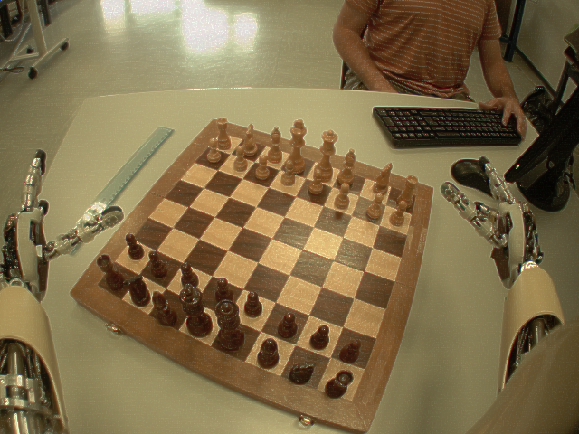
Lines and intersections extracted from the iCub's eyes.

In Part 1 of this post, I discussed my strategy for recognizing the occluded or cluttered chessboards. The main idea was to recast the chessboard recognition problem as an optimization problem. I wrote a Python program that extracts lines and intersections from the video images out of the iCub's eyes. An example of these lines is shown to the right. I developed a scoring function that takes a set of four points representing the corners of a quadrilateral and assigns a high number to quadrilaterals that seem to match a chessboard, and a low number to those that don't. This scoring function does a reverse perspective projection and checks to see if the warped image matches the criteria from the last post:

1. What percentage of the expected horizontal and vertical grid lines are matched?
2. What percentage of the grid intersection points are matched?
3. How uniform is the color is the fringe just outside of the warped image?

Now we have a fitness function (also known as an objective function or cost function) that can score each proposed chessboard. We can use a black-box optimization method to find the chessboard that scores best. Specifically, we will use an evolutionary algorithm. These methods are described in this post, and the actual solution is discussed in Part 3.

Black-box Optimization

A black-box optimization method is given a fitness function with no extra information. The fitness function is just a black-box, an engineering term for a component in a design that reliably does some work without the designer needing to know how it works. The fitness function will give no other information other than the value of search point. A black-box optimizer searches through the inputs to the fitness function trying to find points with high scores.

Gradient-based (Newton) Methods

Black-box optimization was originally named to contrast with the gradient-based or Newton methods that everyone learns in high-school calculus. A gradient-based method method not only sees the fitness value \(f(x)\), it also sees the gradient \(\nabla f(x)\), the direction in which the fitness increases most rapidly. Newton methods can find the high and low points of a function very quickly because they are given good information about where to look next. Conjugate gradient Ascent reduces error with the square of time. That is, if at time \(t = 1\) the different in current fitness from the highest nearby fitness value is \(100\), then at time \(t=2\) will be \(10\), at least in theory. 

But there are caveats. First, Newton methods need a gradient. In a case like ours, the fitness function is a program, and you can't take the derivative of a program. You could extract a math formula from the program with a lot of hard work. And in this case, that formula would even be differentiable (it's piecewise linear by design). But it would take many symbols to write it down.  It would be much easier to estimate the gradient by \(\frac{1}{2} \left(f (x + h) - f(x-h)\right) \) using small increments \(h\) in each direction. However, estimated gradients slow down gradient ascent so that it only reduces error at a rate proportional to the time -- estimating the gradient costs a linear factor. Not only that, but even with a gradient, some functions don't work very well with gradients. Like ours.

Our scoring function is \(multi-modal\). If you could plot the fitness values over a plane, you would see lots of bumps distributed at the grid points. This is because if you slide the correct quadrilateral for the chessboard over one square, you would still have \(\frac{7}{8}\) of the grid points matched. So in ideal conditions the landscape of our fitness function has a large pyramid over the quadrilateral where the best chessboard is. Then it at each grid points in a box around the correct quadrilateral it has a slightly smaller pyramid, followed by a another row of pyramids at the next grid point, and so on out to the edges of the board. There is also noise created by extraneous and missing lines and intersections. 

If you run a gradient method on this type of fitness function, you will at best get the tip top of one of the small pyramids. Although Newton methods are very accurate, they are local. They don't look for the highest point anywhere in the fitness function, just for the one nearest to the starting point. There are hacks like momentum factors that can avoid small local optima. But if all you have is a regular series of local optima, they won't work.  

Quasi-Newton and Local Methods

The need for non-gradient methods became apparent from the earliest days of computing, and some were even used by some scientists in the Manhattan Project. By the 1960's a number of such methods had been developed -- Compass Search, Powell's method, and the Nelder-Mead (or amoeba) method are three well-known ones. Researchers within the mathematical community call such methods Direct Search. But these methods were not always reliable, and mathematicians disliked the fact that such methods can fail to find even a local optimum in some cases. Instead, they developed quasi-Newton methods such as the BFGS method that provide local convergence guarantees using sophisticated estimation of the gradient. 

Still, estimating gradients is not enough to solve multi-modal and noisy problems, and so direct search methods were researched further. Starting from the Nelder-Mead algorithm, Virginia Torczon and her colleagues have developed a much improved method called pattern search.  One nice thing about pattern search is that there are (local) convergence proofs and the convergence rates are known. A general pattern search method performs comparably to the best evolutionary algorithms mentioned below (e.g. CMA-ES, Differential Evolution). However, none of these work as well as the simple method that we will ultimately develop by using the characteristics of the chessboard problem, so no more needs to be said about pattern search here.

Evolutionary Algorithms

In Europe during the 1960s, Hans-Paul Schwefel and Ingo Rechenberg developed a method called evolution strategies inspired by Darwinian selection to search for the optima of real functions in Euclidean spaces. In their method, several search points (a population) are placed randomly in the space. A small selection of the best points are then varied in many ways by adding a Gaussian random variable to create a new population. The process is repeated as long as desired. There are no convergence guarantees, but the method can work well, and numerous improvements and variations have been developed over the years.

Around the same time in America, John Holland developed a similar method for binary codes inspired by Mendelian genetics. He called his method a genetic algorithm and published a widely read book named Adaptation in Natural and Artifical Systems in 1975. His student, David Goldberg, popularized these methods in the 1980s, and together with neural networks the terms became widely known in popular science and sci-fi circles.

A genetic algorithm is characterized by a gene encoding, in which solutions to a problem are expressed typically in a binary form as a list of ones and zeros. So to search for solutions to a problem in the real numbers, one might use a fixed decimal encoding. For the integers, one could use two's complement binary numbers. Since any representation inside a computer requires a binary code, genetic algorithms can be easily applied to any object in a digital computer (not necessarily with success).

The other prominent feature of genetic algorithms is crossover. In crossover, two gene encodings are mixed according to some scheme to create a third new gene encoding. Overall, genetic algorithms, like evolution strategies, propose a population of search points, then use the scores to generate a new population using selection, crossover, and mutation. Selection chooses the best points by fitness to generate the next population. Crossover mixes and matches these points, and mutation randomly flips a small number of bits. Populations are generated in this way as long as needed, usually until the population consists of several copies of the same point.

These days, standard genetic algorithms and evolution strategies have been amplified, extended an modified in numerous ways to produce an entire academic field of evolutionary computation, or natural computation. There are optimization methods inspired by the foraging behavior of ants, the migration of geese, and the adaptive defense mechanisms of the immune system. 

Performance of Evolutionary Algorithms

A key characteristic of both evolution strategies and genetic algorithms is that neither provides any guarantees at all with respect to performance. They can and often fail badly, especially when applied to problem naïvely. For this reason, and because of overstated claims by some supporters, these methods have acquired an unwarranted bad reputation in some circles. Nonetheless, they can work quite well if applied with care. Evolutionary algorithms have been used to design a control system for a finless rocket, to evolve a better radio antenna, and to schedule courses satisfying many constraints. 

The study of when and why evolutionary methods work is relatively young. The earliest attempt at explaining behavior was John Holland's schema theory. However, schema theory is not taken seriously anymore, for good reasons. Kenneth de Jong did early experimental work examining when and why genetic algorithms fail.  

Since the mid 1990s, several researchers have begun to study the performance characteristic of evolutionary methods from a formal mathematical point of view. Some success and failure cases are now known. For example, needle in a haystack problems cannot be solved without exponential time. And a simple evolution strategy performs better than line search on on the problem of finding an exact match to some unknown string of bits. But theory that is known lags quite far behind practice. One important fact is that the No Free Lunch theorems imply that there must be a class of problems for which evolutionary methods perform better than gradient methods. It is a fallacy to say that because gradient methods are understood they must perform better! But it is also a fallacy to assume that the class of problems exists where evolutionary methods perform better is likely to occur in real-world problems. Still, evolutionary methods are used because they can work well.

In practice, the best evolutionary methods at present for searching real functions seem to be Differential Evolution and CMA-ES (or its generalized version, NES). Both of these methods tend to perform well out of the box, comparably to the pattern search mentioned above. And any of those three are far superior to a Newton or quasi-Newton method on certain multi-modal problems (like the chessboard problem). Differential evolution has even been shown to converge to the global optimum under certain conditions. 

But to really get a good evolutionary algorithm, one has to take problem characteristics into account. In a way, this defies the original plan for a black-box method. The idea was that we would get good performance on any problem. But the reality is that one gets good performance on some problems by ignoring others. There is a general tradeoff between generality and quality/speed. In a recent paper, I even showed what the optimal solutions look like when you have a model of fitness problems. The catch is that the optimal solution averages over problems (and includes a second internal optimization). So a general model has to average over problems that aren't be solved at the moment, for which it sacrifices some performance on problems that are being solved.

Thus if you really want to solve a problem, you have to tinker with the method. One interesting thing about the evolutionary framework is its flexibility. One has two very flexible phases, selection and mutation. The selection phase uses fitness values in order to decide which search points should receive focus, and the mutation phase then tries to combine or alter the selected points to potentially make them better. After choosing a good general selection method, such as tournament selection or even evolutionary annealing, one can adapt the mutation process to match the search problem at hand. One way to manage such adaptations is by using fancy indirect encodings, or one can work directly in the search space using complex mutators.

Our chessboard recognition algorithm will do exactly this: it will directly search quadrilaterals, using the known features of the problem to choose good mutations. In this way, we will be able to find chessboards much faster than any general-purpose method does while still using an evolutionary algorithm. But that is the topic for the next post.

Robust Chessboard Recognition, Part 1: Some Tools

Raw image of chessboard from iCub's left eye.

In order for the iCub to play chess, it first needs to see the board. For eyes, the iCub has two Dragonfly cameras with VGA resolution (640 x 480) that produce 30 frames per second. An example frame with the chessboard in it is shown to the right. It might seem easy to figure out where a chessboard is inside of an image. After all, checkerboard patterns are commonly used to calibrate cameras for image processing.  It is true that it is easier to locate the chessboard in an image than it is to solve than many of the other problems we will encounter, but as we will see, it is by no means simple or straightforward to do so.

To find the chessboard, we will use computer vision techniques to extract information about the image. We could use more advanced techniques, such as neural nets, but they are not needed to get a good solution. If we wanted to train a neural network to find the board using supervised techniques (e.g. backpropagation), we would need to gather a large dataset of chessboard images, either by generating images or by collecting and annotating hundreds of thousands of frames from the robot. If we generate the images, then we can't be sure that the learning will transfer from generated images to the real frames. Collecting the images would take many weeks of thankless labor. As an alternative, one could try to use the inherent properties of chessboard images in order to develop an unsupervised training method, but there is no obvious way to do so in this case. So rather than make this task more complicated than it needs to be, we'll just use standard methods for detecting lines and intersections.

Undistorting the Image

Image of chessboard after removing lens distortion.

Take a look at the image from the robot's cameras. Notice that the lines in the picture are not straight; the raw images are distorted by the camera lens. This distortion needs to be removed so that we can extract the lines.  Thanks to the many high-powered methods available in the open source computer vision package Open CV, the distortion can be taken out by just one call to the undistort method once we know the parameters for the camera lens. As discussed here, these parameters can be extracted by another call to a function named findChessboardCorners, which requires nothing more than an image with a chessboard in it as input. The undistorted image is shown to the right.

At this point, you might wonder whether we can just call findChessboardCorners on our raw image and be done with the chessboard recognition problem. The answer, of course, is no. While findChessboardCorners is good at finding unobstructed chessboards that are roughly parallel the frustrum of the camera, it fails utterly when the chessboard is covered with chess pieces and laying at an oblique angle on a table. But this is exactly the situation for which we need to solve the problem, so we have to develop our own method.

Our Strategy to Find the Chessboard

We will use the following properties of the chessboard to develop a robust detection method for chessboards:

1. Chessboards are square.
2. Chessboards contain a grid of 9 horizontal and vertical lines, equally spaced.
3. Chessboards contain an 9 x 9 grid of intersections from these lines, again equally spaced.
4. Chessboards typically have a monochrome fringe with no lines around the board.
5. The 64 squares in a chessboard alternate in color, with one dark and one light color.

Chessboard after perspective warp given the board outline.

Many of these statements (such as equally spaced, horizontal, and vertical) require the robot to be looking at the chessboard from directly overhead at a known distance from the board. Since we don't know where the board is, that's too much to ask. However, we know that the chessboard is a square and that its position in the image is determined by a perspective projection from 3D into 2D space, and given any quadrilateral in an image, we can compute the perspective transformation required to warp the quadrilateral back into a square viewed from directly overhead at a known scaling. In fact, Open CV provides us with a function getPerspectiveTransform that does exactly what we want, giving us a 4x4 matrix that we describes the perspective transform (we could also use findHomography, but we're not going to need it). We can "undo" the perspective transformation in order to flatten the chessboard by using warpPerspective. If we knew the quadrilateral outlining the chessboard, then we would get an image like the one to shown here. We would see that the warped image roughly satisfies the five observations about chessboards listed above. 

Of course, we don't know the outline of the chessboard yet, but there's nothing that prevents us from guessing. We could pick any four points in the image that outline a (convex) quadrilateral, undo the perspective transform, and then visually check items 1-5 listed above. Since there are 94,371,840,000 possible outlines of our chessboard, we can't check every quadrilateral, but we could easily check at least some of them. We could check even more if we could find an automated way of checking items 1-5. If we write a program that is smart about how to pick points to check, it might even be able to find the chessboard fast enough to be useful. And that is what we will do, using a custom-built evolutionary algorithm. 

But that's the topic for the next post. In this post, we'll finish off by describing the tools we need in order to check whether a proposed outline of a chessboard is a good outline or not.

Processing Chessboard Images

Chessboard edges detected by Canny edge detector.

The chessboard features listed above were chosen to depend on lines, intersections, and colors. It's easy to see how we can get colors out of an image, but lines and intersections are more difficult. We start off by extracting edges using a Canny edge detector. Edge detectors try to find areas in an image where colors change rapidly. These areas are likely to indicate where one object begins and another ends. They could also indicate color patterns on a single object. We hope to detect the boundaries between chessboard spaces as edges. The picture to the left shows what the Canny edge detector does to our undistorted chessboard image (using Open CV's canny function, after various successive calls to erode and dilate). As expected, the chessboard shows through clearly in the edges, although many edges are chopped up by the chess pieces.

Now we need to pass from edges to lines. The traditional tool for this purpose is the Hough transform, which scans through the image searching for lines at each possible angle. Using the probabilistic version HoughLinesP in Open CV, we get a list of dozens of potential lines satisfying given thresholds on length, etc. These lines will be used to check items 2 and 4 in the list of chessboard features above.

We can easily compute the intersection points of each pair of lines using some basic vector math. However, if there are hundreds of lines, there are tens of thousands of possible intersections, so it's important to be very careful about how we do this. I used numpy to compute all of the intersections in parallel using matrix operations in a matter of milliseconds thanks to built-in hardware acceleration. If we were to loop through all pairs of lines explicitly, it would take far longer. Careful thresholding on the Hough transform is also useful to cut down on the number of lines.

Chessboard with lines and intersections from Hough transform.

All of the intersections give us a long list of points. We keep only the intersection points that intersect inside of the line segments that generated the intersection, and throw away the rest. In addition to these intersection points, we add in the endpoints of each line segment, which may represent an intersection that the edge detector failed to see. These points are candidates for the grid intersections and can be used to check item 3 on the list of chessboard features.

The lines, their intersections, and endpoints are shown to the right, with lines in red and intersections as white circles. The chessboard is clearly visible, but it is also missing some intersections and grid lines. Thus when we match the chessboard, we will have to allow for the possibility that some elements of the chessboard are invisible to us. We are looking for the candidate chessboard that has as many of the desired features as possible.

Chessboard after color filtering to reveal dark and light squares.

As a final step, we can threshold the colors in order to try to discriminate light squares from dark squares as in item 5 of our chessboard features. A picture is shown to the left. Notice that the colors are not reliable; dark pieces on light squares can cause confusion, and our threshold is not perfect. The colors would also fail if our chessboard had different colors or were placed in different lighting. Additionally, computing a score for the color is more computationally expensive than the other steps. For these reasons, we only use the color to select among the best potential chessboards.

Chessboard Detection as an Optimization Problem

Putting the information above together (and omitting some details), we can build a scoring function for potential chessboards. The scoring function takes a quadrilateral \(q\) and warps the image to remove the perspective transform so that the edges of the quadrilateral are located at \(xy\)-coordinates \((-N,-N)\), \((-N,N)\), \((N,N)\), and \((N,-N)\) for some \(N\) (we used \(N=480\) to avoid certain precision issues with Open CV). Then it computes three subscores:

1. The percentage of horizontal and vertical lines of the chessboard that are matched.
2. The percentage of intersection points on the chessboard that are matched.
3. The variation in a fringe of width $N\slash 16$ around the chessboard. 

The first two components give 'partial credit' for lines that are not quite straight and points that are not quite at the intersections; this credit scales with the square of the error in the line angle or the intersection error. This is done so that the score behaves smoothly around the good matches, leading a chessboard search along a smooth path to the best matches. For the line and intersection subscores, the "percentages" may be greater than one, because some lines and points may overlap. The variation of the fringe is simply the sum of the squared differences from the average color, times a scaling factor. 

Thanks to an efficient implementation, plus Open CV's support for offloading items such as perspective warping to our nVidia 780ti graphics card, our score function can be computed in about 200 microseconds. So we can test 5,000 possible chessboards per second. Although we still cannot check all of the billions of possible boards, with a good heuristic choice, we can find very good matches in a matter of seconds. 

As often happens in artificial intelligence problems, our chessboard recognition effort has now led us to an optimization problem. Specifically, we want to find the quadrilateral in the image that results in the best chessboard after we warp it to take out the perspective transform. If \(Q\) is the set of potential quadrilaterals and \(score\) is our scoring function, then we want to choose the quadrilateral \(q\) such that $$q = \mathrm{arg\,min}_{q' \in Q} \,\,score(q').$$ The problem of detecting the chessboard is now reduced to the problem of optimizing the \(score\) function using whichever method works best.

Conclusion

Chessboard detected using our evolutionary algorithm.

Some final comments are in order about why we are solving the problem in such a roundabout manner. After all, it might seem that it would be easier to use a brute force approach (such as the one used to detect chessboards for calibration). For example, we could use the lines in order to detect possible rectangles, and then assemble sets of similar rectangles hierarchically into a chessboard pattern. But in practice, the rectangle-based method is far slower than the ones we have outlined. There are billions of possible rectangles, and it would be difficult to choose which ones to prefer. In the end, our optimization method works quickly and is correct in most instances. It seems doubtful that there is a simpler method for robust chessboard detection that works faster and more elegantly. I would actually prefer to have a board recognition method based on a convolutional neural network (a more complex method), but at this point I am not quite sure either how to get good training data for the network or how to find a good unsupervised training method (I have tried a few approaches).

In the next post, I'll discuss the evolutionary method that we developed and the other optimization methods that we could have chosen. 

Welcome and Introduction

The iCub waves hello.

Meet the iCub.

The iCub was designed by the folks at the Italian Institute of Technology in Genoa with the goal of creating a robot platform with the general physical characteristics and capabilities of the toddler. Under the tutelage of the brightest minds in Europe, the iCub would learn to crawl, babble, and play with blocks. So far, at least 20 iCubs have been built; they live in various research labs across Europe. This iCub lives in Lugano, Switzerland at the Dalle Molle Institute of Artificial Intelligence Studies.

And now, this iCub is going to take on a task that few toddlers ever accomplish: he's going to learn to play chess. That's where I come in. In 2013, I received a grant from the US National Science Foundation (NSF) to spend two years in Lugano teaching the iCub to play chess.

It may seem rather esoteric and impractical to teach a robot to play chess. After all, aren't there more interesting problems to solve? Shouldn't I be teaching a robot to operate on cancer patients or bravely venture into the site of a nuclear reactor meltdown?

But despite the seemingly trivial setting, the problem of making a robot play chess cuts through to the core of some very hard problems in robotics. Industrial robotics have been successful in manufacturing for over a generation, but only because it is possible to strictly control the environment they work in. Move an important bolt a few centimeters to one side, and the car door falls off before it ever leaves the factory floor.

Thus we speak of autonomous robotics, by which we mean robots that can operate in unpredictable settings, like your grandmother's kitchen. There have been a lot of advances in this area too - many households have been vacuumed by small autonomous robots. But these robots do simple tasks in a simple way. To do more complex tasks, a robot really needs to be able to perceive the world around it and act reliably based on its perception.

"But what about self-driving cars?", you ask, "Aren't they able to perceive the world?" Well, a lot of advances have been made in this area over the last decade, and in fact such cars do perceive the world very well using a combination of digital cameras and laser range-finders. But when you think about the controls on a car, they are really quite simple: you can turn the wheels, punch the accelerator, or hit the brakes. That's about it. Just three factors to control.

The iCub, however, has 16 motors in each arm, 6 in its head, 3 in the torso, and 5 in the legs. That's 41 factors that have to be controlled, and with sufficient coordination that the robot doesn't fall forward when he reaches his arm out. Although it's easy to predict what will happen when a car turns its wheels, it's not so easy to say whether moving 16 motors in a certain way will put a robot arm in a position to pick up a chess piece. In autonomous robotics, perceptual tasks have been studied much more deeply than the control of robots with lots of motors. It's not really known how to make consistent, smooth motions with a robot arm once it has more than a few degrees of freedom. Sure, there are lots of approaches, such as rapidly expanding random trees or solving calculus of variations problems. But the problems are just hard (see here for example of what it takes to get a humanoid walking). If you want a robot to fry up an omelette for breakfast, you need technologies that are far more advanced than a self-driving car.

So why chess? Well, to play chess, the iCub has to find the board (even when it's covered by pieces or blocked by a hand) and identify where the pieces are, which may require moving his head around a bit to get a better view of each piece. Then, the iCub has to coordinate all of its motors to pick up a single chess piece surrounded by other pieces without knocking anything over. It has to move the chess piece without dropping it, and set it down without further disturbing the board. Each one of these problem is difficult to solve. But if they can be solved, getting your personal robot to bring you a fried omelette in bed may be one step closer to reality.

So that's what I've been working on for the last year. I have one more year left in this project, and as time goes by, I'll be posting pictures of the iCub's progress and explaining the issues involved in the design. So sign up to follow this blog, and watch as the iCub's chess game improves!